The point of this handout is to illustrate some basic points about
product and cost curves. Below, we will address various ways of
measuring output and learning how factors contribute to producing that output.
When we measure the cost of production, we'll want to make some similar
calculations there.
Product Curves
Consider the table below. The table assumes that a certain good is
produced by using labor and capital (K), where varying amounts
of labor are hired to work with a fixed amount of capital (4 units).
For the sake of this example, let's assume that these 4 units of capital
are 4 pieces of equipment (e.g. 4 machines).
Each combination of labor (L) and capital (K) produces a different
level of output (Q). Eventually, however, adding laborers adds
nothing to output and will even actually decrease output if more
laborers were hired. Once we know the output, it is possible to
determine how our variable factor contributes to the production of
that output. To do so, we calculate the average product of labor (APL)
and marginal product of labor (MPL) by computing Q/L and DQ/DL respectively.
|
L |
K |
Q |
APL |
MPL |
|
0 |
4 |
0 |
- |
- |
|
1 |
4 |
10 |
10 |
10 |
|
2 |
4 |
36 |
18 |
26 |
|
3 |
4 |
60 |
20 |
24 |
|
4 |
4 |
80 |
20 |
20 |
|
5 |
4 |
90 |
18 |
10 |
|
6 |
4 |
96 |
16 |
6 |
|
7 |
4 |
98 |
14 |
2 |
|
8 |
4 |
98 |
12.2 |
0 |
|
9 |
4 |
90 |
10 |
-8 |
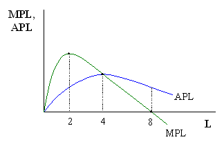
If we take this information and insert it into a graph, we have:

The graph shows several points where the relative position of the average and marginal product curves tell us something about how the average product of labor is changing. This illustrates the average-marginal rule where when a marginal value is less than (greater than) an average value, the average is falling (rising). When the two are equal, the average is constant - which implies that the average should be at a maximum or minimum point. On the graph, we see that when 4 units of labor are hired, MPL = APL and APL is at a maximum. When 2 units (8 units) are hired, APL < MPL and APL is rising (APL > MPL and APL is falling).
Cost Curves
Now, suppose we assume that this firm must pay $20 for each unit of
labor hired, and $25 for each unit of capital purchased. This information
allows us to take the data from the table above and measure (economic)
costs. The total cost of the variable factor and total cost of the fixed
factor (i.e. Total Variable Cost, TVC, and Total Fixed Cost, TFC) add
up to the (overall) Total Cost, TC.
Just as we calculated average and marginal product above, we can calculate
the average (total) cost and marginal cost here. Average Cost, AC, is
calculated by dividing total cost by output (i.e. TC/Q). Marginal
Cost, MC, is calculated as the change in total cost caused by
a change in output (i.e. DTC/DQ).
|
L |
K |
Q |
TVC |
TFC |
TC |
AC |
MC |
|
0 |
4 |
0 |
0 |
100 |
100 |
- |
- |
|
1 |
4 |
10 |
20 |
100 |
120 |
12.00 |
2.00 |
|
2 |
4 |
36 |
40 |
100 |
140 |
3.89 |
0.77 |
|
3 |
4 |
60 |
60 |
100 |
160 |
2.67 |
0.83 |
|
4 |
4 |
80 |
80 |
100 |
180 |
2.25 |
1.00 |
|
5 |
4 |
90 |
100 |
100 |
200 |
2.22 |
2.00 |
|
6 |
4 |
96 |
120 |
100 |
220 |
2.29 |
3.33 |
|
7 |
4 |
98 |
140 |
100 |
240 |
2.45 |
10.00 |
|
8 |
4 |
98 |
160 |
100 |
260 |
2.65 |
- |
|
9 |
4 |
90 |
180 |
100 |
280 |
3.11 |
- |
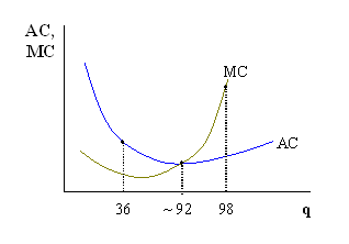
As above, we can take the information from the table and draw the
graph of average and marginal cost:

Just as above, we see the average-marginal rule at work when comparing the AC and MC curve at 36 and 98 units of output. When AC = MC, at about 92 units of output, AC is at a minimum point.